Plot NCATS-sol

This tutorial runs the PSMA workflow on the NCATS-sol classification dataset and renders the static and interactive posterior plots.

The dataset uses low_solubility as a binary endpoint: class 1 means low solubility and class 0 means moderate-to-high solubility.

Imports

The tutorial uses the pure computation API, so no PSMA artifacts are written to disk.

from pathlib import Path
import sys

import matplotlib.pyplot as plt
import numpy as np
import pandas as pd
from bokeh.embed import file_html
from bokeh.resources import CDN
from IPython.display import HTML

for candidate in [Path.cwd(), *Path.cwd().parents]:
    if (candidate / "psma").is_dir():
        sys.path.insert(0, str(candidate))
        break

from psma import compute_psma_surface  # noqa: E402
from psma.plot import (  # noqa: E402
    plot_posterior_2d,
    plot_posterior_2d_interactive,
    plot_posterior_3d,
)

Load the tutorial data

The CSV is stored with the documentation because it supports this tutorial directly.

def find_data_path() -> Path:
    """Find the NCATS-sol CSV from common notebook execution roots."""
    candidates = [
        Path("docs/_data/solubility_NCATS-sol.csv"),
        Path("_data/solubility_NCATS-sol.csv"),
        Path("../_data/solubility_NCATS-sol.csv"),
    ]
    for candidate in candidates:
        if candidate.exists():
            return candidate
    raise FileNotFoundError("Could not find solubility_NCATS-sol.csv")


df = pd.read_csv(find_data_path())
df = df.loc[:, ["canonical_smiles", "low_solubility"]].dropna()
df["canonical_smiles"] = df["canonical_smiles"].astype(str).str.strip()
df = df.loc[df["canonical_smiles"] != ""].copy()
df["low_solubility"] = pd.to_numeric(df["low_solubility"], errors="raise").astype(int)
df = df.drop_duplicates(subset="canonical_smiles", keep="first").reset_index(drop=True)
df.insert(0, "mol_id", [f"ncats_sol_{index:05d}" for index in range(len(df))])

df.head()

	mol_id	canonical_smiles	low_solubility
0	ncats_sol_00000	O=c1cc(-c2ccc(O)c(O)c2)oc2cc(O)cc(O)c12	0
1	ncats_sol_00001	C=CCc1ccc(O)c(-c2ccc(O)c(CC=C)c2)c1	0
2	ncats_sol_00002	CC[C@H]1NC(=O)[C@@H](NC(=O)c2ncccc2O)[C@@H](C)...	0
3	ncats_sol_00003	O=c1ncn2nc(Sc3ccc(F)cc3F)ccc2c1-c1c(Cl)cccc1Cl	0
4	ncats_sol_00004	O=C(Cc1ccc(Cl)c(Cl)c1)Nc1ccc(S(=O)(=O)Nc2ccon2...	0

df["low_solubility"].value_counts().sort_index().rename("count")

low_solubility
0    1054
1    1399
Name: count, dtype: int64

Run PSMA without writing artifacts

The dataset is already binary, so label_threshold=0.5 with label_direction="ge" preserves the 0/1 class labels.

def run_ncats_sol(split_method: str):
    """Compute one NCATS-sol PSMA result without writing artifacts."""
    return compute_psma_surface(
        df,
        y_col="low_solubility",
        smiles_col="canonical_smiles",
        mol_id_col="mol_id",
        similarity_method="rdkit_morgan_tanimoto",
        split_method=split_method,
        butina_distance_cutoff=0.4,
        label_threshold=0.5,
        label_direction="ge",
        test_fraction=0.2,
        random_state=7,
    )


random_result = run_ncats_sol("random")
butina_result = run_ncats_sol("butina")

Projection diagnostics flagged instability with rank=1957 cond=3.9070720654275174e+19

Projection diagnostics flagged instability with rank=1958 cond=1.9596175125530284e+19

pd.DataFrame(
    {
        "split": ["random", "butina"],
        "auc": [random_result.metrics.auc, butina_result.metrics.auc],
        "mcc": [random_result.metrics.mcc, butina_result.metrics.mcc],
        "train_n": [len(random_result.indices.train), len(butina_result.indices.train)],
        "test_n": [len(random_result.indices.test), len(butina_result.indices.test)],
    }
)

	split	auc	mcc	train_n	test_n
0	random	0.652273	0.226285	1962	491
1	butina	0.634628	0.213330	1962	491

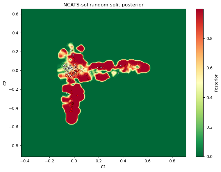
Static 2D posterior plot

The 2D view is the most compact summary of the posterior surface and projected test compounds.

fig, ax = plt.subplots(figsize=(8, 6))
plot_posterior_2d(
    ax,
    grid_x=random_result.grid.grid_x,
    grid_y=random_result.grid.grid_y,
    posterior_z=random_result.grid.posterior_z,
    pos_density_z=random_result.grid.pos_density_z,
    c_test=random_result.coords.c_test,
    y_test_bin=random_result.labels.y_test_bin,
)
ax.set_title("NCATS-sol random split posterior")
fig.tight_layout()

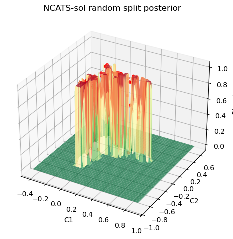
Static 3D posterior plot

The 3D view makes the geometry of the posterior surface easier to inspect.

fig3d, ax3d = plot_posterior_3d(
    grid_x=random_result.grid.grid_x,
    grid_y=random_result.grid.grid_y,
    posterior_z=random_result.grid.posterior_z,
    c_test=random_result.coords.c_test,
    prob_test=random_result.prob_test,
)
ax3d.set_title("NCATS-sol random split posterior")
fig3d.tight_layout()

Interactive posterior plot

The interactive plot adds toggleable layers, contour-level hover, compound-level hover metadata, and RDKit hover depictions from SMILES.

test_mol_ids = random_result.frames.test["mol_id"].astype(str).to_numpy()
smiles_by_mol_id = dict(
    zip(df["mol_id"].astype(str), df["canonical_smiles"].astype(str), strict=True)
)
test_smiles = np.asarray(
    [smiles_by_mol_id[mol_id] for mol_id in test_mol_ids], dtype=object
)

interactive_plot = plot_posterior_2d_interactive(
    grid_x=random_result.grid.grid_x,
    grid_y=random_result.grid.grid_y,
    posterior_z=random_result.grid.posterior_z,
    pos_density_z=random_result.grid.pos_density_z,
    c_test=random_result.coords.c_test,
    y_test_bin=random_result.labels.y_test_bin,
    prob_test=random_result.prob_test,
    mol_ids=test_mol_ids,
    smiles=test_smiles,
    width=800,
    height=600,
)
HTML(file_html(interactive_plot, CDN, "Interactive PSMA Posterior"))